
Documentation > Explore
In the following we will use the term of fitness to denote the calibration error function, or calibration criterion. Several types of evaluation functions can be used as fitness. Most of the time, they are either some kind of distance between model dynamics and data, or statistical measures performed on the output dynamics.
The calibration profile method is suited to reveal a model's sensitivity regarding its parameter, hence the highest score possible in sensitivity. However, it does not retrieve information about the input space nor the output space structures, as it focus on one parameter/input, every other input being let free (to be calibrated). As the studied parameter varies, the other parameter are calibrated, so this method scores very well regarding calibration. For the same reason, it can handle stochasticity. Finally, the profile method realizes calibrations on the other inputs for each interval of the input under study, so the more inputs, the more sensitivity to dimensionality of input space.
Run
Given a fitness function, the profile of a selected parameter i is constructed by dividing its interval into subintervals of equal size. For each subinterval, i is fixed, and the model is calibrated to minimise the fitness, similarly to Calibration. The optimisation is performed over the other parameters of the model.
As an example, let's consider a model with 3 parameters i, j and k, each taking real values between 1 and 10. The profile of the parameter i is made by splitting the [1,10] interval into 9 intervals of size 1. Then, calibration is performed in parallel within each subinterval of i.
At the end of the calibration, we obtain sets of i,j and k values minimising the fitness, with i taking values in each subinterval. By plotting the fitness against the values of i, one can visually determine if the model, within each of i subintervals, is able to produce acceptable dynamics.
An important nuance is that for each point of this fitness vs i values plot, fitness values has been obtained by "adjusting" j and k to counterbalance the effect of i's values on the model dynamics. This means that j and k values vary for each point of the i parameter profile plot.
The hook arguments for the
The computed calibration profiles may take very diverse shapes depending on the effect of the parameter of the model dynamics, however some of this shapes are recurrent. The most typical shapes are shown on the figure bellow.
[online version] [bibteX]
Profile parameters 🔗
The profile (or calibration profile) method is designed to test the sensitivity of the input parameters in a calibration context. Calibration profile algorithm differs from traditional sensitivity analysis: it captures the full effect of a parameter variation on the model fitness, every other input being calibrated to optimize the calibration criterion.In the following we will use the term of fitness to denote the calibration error function, or calibration criterion. Several types of evaluation functions can be used as fitness. Most of the time, they are either some kind of distance between model dynamics and data, or statistical measures performed on the output dynamics.
Method's score 🔗
The calibration profile method is suited to reveal a model's sensitivity regarding its parameter, hence the highest score possible in sensitivity. However, it does not retrieve information about the input space nor the output space structures, as it focus on one parameter/input, every other input being let free (to be calibrated). As the studied parameter varies, the other parameter are calibrated, so this method scores very well regarding calibration. For the same reason, it can handle stochasticity. Finally, the profile method realizes calibrations on the other inputs for each interval of the input under study, so the more inputs, the more sensitivity to dimensionality of input space.
Run
Given a fitness function, the profile of a selected parameter i is constructed by dividing its interval into subintervals of equal size. For each subinterval, i is fixed, and the model is calibrated to minimise the fitness, similarly to Calibration. The optimisation is performed over the other parameters of the model.
As an example, let's consider a model with 3 parameters i, j and k, each taking real values between 1 and 10. The profile of the parameter i is made by splitting the [1,10] interval into 9 intervals of size 1. Then, calibration is performed in parallel within each subinterval of i.
At the end of the calibration, we obtain sets of i,j and k values minimising the fitness, with i taking values in each subinterval. By plotting the fitness against the values of i, one can visually determine if the model, within each of i subintervals, is able to produce acceptable dynamics.
An important nuance is that for each point of this fitness vs i values plot, fitness values has been obtained by "adjusting" j and k to counterbalance the effect of i's values on the model dynamics. This means that j and k values vary for each point of the i parameter profile plot.
Profile within OpenMOLE 🔗
Specific constructor 🔗
TheProfileEvolution constructor takes the following arguments:
evaluation: the model task, that has to be previously declared in your script,objective: the fitness, a sequence of output variable defined in the OpenMOLE script that is used to evaluate the model dynamics, to be minimized (for this method it is advised to use a single objective),profile: the sequence of parameter to profile, use in key word to set the number of intervals (e.g. Seq(myParam) or Seq(myParam in 100) or Seq(myParam in (1.0 to 5.0 by 0.5))),genome: a list of the model input parameters with their values interval declared with theinoperator,termination: a \"quantity\" of model evaluation allocated to the profile task. Can be given in number of evaluations (e.g. 20000) or in computation time units (e.g. 230 minutes, 2 days...),parallelism: optional number of parallel calibrations performed within i subinterval, defaults to 1,stochastic: optional the seed provider, mandatory if your model contains randomness,distribution: optional computation distribution strategy, default is \"SteadyState\".accept: (optional) a predicate which must be true for genomes that can be accepted by the genome sampler (for instance \"i1 > 50\").
Hook 🔗
The output of the genetic algorithm must be captured with a hook which saves the current optimal population. The generic way to use it is to write eitherhook(workDirectory / "path/of/a/directory") to save the results as CSV files in a specific directory, or hook display to display the results in the standard output.
The hook arguments for the
ProfileEvolution are:
output: the file in which to store the results,keepHistory: optional, Boolean, keep the history of the results for future analysis,frequency: optional, Long, the frequency in generations where the result should be saved, it is generally set to avoid using too much disk space,keepAll: optional, Boolean, save all the individuals of the population not only the optimal ones.
Use example 🔗
To build a profile exploration, use theProfileEvolution constructor.
Here is an example :
val param1 = Val[Double]
val param2 = Val[Double]
val fitness = Val[Double]
val mySeed = Val[Long]

ProfileEvolution(
  evaluation = modelTask,
  objective = fitness,
  profile = param1,
  genome = Seq(
      param1 in (0.0, 99.0),
      param2 in (0.0, 99.0)
  ),
  termination = 2000000,
  parallelism = 500,
  stochastic = Stochastic(seed = mySeed, sample = 100)
) by Island(10 minutes) hook(workDirectory / "path/to/a/directory")
Interpretation guide 🔗
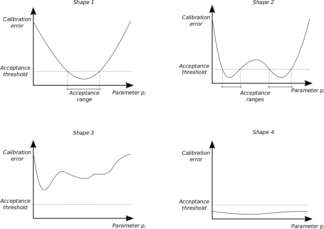
A calibration profile is a 2D plot with the value of the profiled parameter represented on the X-axis and the best possible calibration error (i.e. fitness value) on the Y-axis. To ease the interpretation of the profiles, we define an acceptance threshold on the calibration error (i.e. fitness). Under this acceptance threshold, the calibration error is considered sufficiently satisfying and the dynamics exposed by the model sufficiently acceptable. Over this acceptance threshold the calibration error is considered too high and the dynamics exposed by the model are considered unacceptable, or at least non-pertinent.The computed calibration profiles may take very diverse shapes depending on the effect of the parameter of the model dynamics, however some of this shapes are recurrent. The most typical shapes are shown on the figure bellow.
- Shape 1 occurs when a parameter is constraining the dynamic of the model (with respect to the fitness calibration criterion). The model is able to produce acceptable dynamics only for a single specific range of the parameter. In this case a connected (i.e. \"one piece\" domain) validity interval can be established for the parameter.
- Shape 2 occurs when a parameter is constraining the dynamic of the model (with respect to the fitness calibration criterion), but the validity domain of the parameter is not connected. It might mean that several qualitatively different dynamics of the model meet the fitness requirement. In this case, model dynamics should be observed directly to determine if every kind of dynamics is suitable or if the fitness should be revised.
- Shape 3 occurs when the model \"resists\" to calibration. The profile does not expose any acceptable dynamic according to the calibration criterion. In this case, the model should be improved or the calibration criterion should be revised.
- Shape 4 occurs when a parameter does not constrain sufficiently the model dynamics (with respect to the fitness calibration criterion). The model can always be calibrated whatever the value of the profiled parameter. In this case this parameter constitute a superfluous degree of liberty for the model : its effect is compensated by a variation of the other parameters. In general it means that either this parameter should be fixed, or that a mechanism of the model should be removed, or that the model should be reduced by expressing the value of this parameter as a function of the other parameters.
[online version] [bibteX]


