Documentation > Tutorials
 Run
Run
The Fire model integration has been covered in the NetLogo page of the Model section, so we take it from here. The former script was already performing a sensitivity analysis, by varying @code{density} from 20 to 80 by step of 10, with 10 replications for each ( The change of regime clearly appears between 50% and 75% percent density, so we are going to take a closer look at this domain: we change the exploration task to have the density taken from 50% to 75% by step of 0.1%, still with 10 replications:
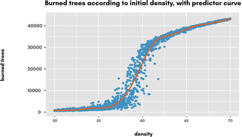 The trend appears to be a sigmoïd shape on which we could find the mid point, the steepness of the curve and so on, to better characterize the phenomenon.
Eventually, let's have a look at the stochasticity of the model. Looking at the plot, we see that there is a lot of variation possible, especially in the transition zone, around 60% density. Let's make a final exploration task to investigate the variation of model outputs for several replications of the same parameterization. We now take densities within [50;70] and take 100 replications for each: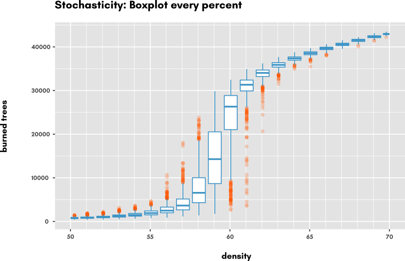 As we can see, stochasticity has a huge effect right in the middle of the transition of regime, reaching its maximum at 59%.
Another interesting thing to investigate would be the density from which the fire propagates to the end of the zone (right side of NetLogo World).
A slight modification of the model code would do the trick, hint: @code{any? patches with-max [pxcor] ...} would be a good starting point :-) but we let you do it on your own (any successful attempts would win the right to be displayed right here!).
As we can see, stochasticity has a huge effect right in the middle of the transition of regime, reaching its maximum at 59%.
Another interesting thing to investigate would be the density from which the fire propagates to the end of the zone (right side of NetLogo World).
A slight modification of the model code would do the trick, hint: @code{any? patches with-max [pxcor] ...} would be a good starting point :-) but we let you do it on your own (any successful attempts would win the right to be displayed right here!).
For completeness sake, here is the R code snippet to produce plots from a CSV export of your results file (RStudio version 1.0.153, ggplot2 version 2.2.1). The result files correspond to the experiments above in the same order.
Content:
Sensitivity analysis 🔗
Typical sensitivity analysis (in a simulation experiment context) is the study of how the variations of an input affects the output(s) of a model.
Run
Prerequisites 🔗
A plugged model in OpenMOLE: see Step By Step IntroductionVariation of one input 🔗
The most simple case to consider is to observe the effect of a single input variation on a single output. This is achieved by using an @b{exploration task}, which will generate a sequence of input values, based on its given boundaries, and discretisation step.val my_input = Val[Double]
val exploration =
ExplorationTask(
(my_input in (0.0 to 10.0 by 0.5))
)Real world example 🔗
theFire.nlogo model is a simple, one-parameter, simulation model that simulates fire propagation.
This model features a threshold value in its unique parameter domain, below which fire fails to burn the majority of the forest, and beyond which fire propagates and burns most of it.
We will perform sensitivity analysis to make this change of regime appear.
The Fire model integration has been covered in the NetLogo page of the Model section, so we take it from here. The former script was already performing a sensitivity analysis, by varying @code{density} from 20 to 80 by step of 10, with 10 replications for each (
mySeed has 10 different values for each value of density).
In our case, the quantum of 10 percent is quite coarsed, so we make it 1 percent:
val exploration =
  ExplorationTask(
    (density in (20.0 to 80.0 by 1.0)) x
    (mySeed in RandomSequence[Int](size = 10))
  )
val exploration =
  ExplorationTask(
    (density in (50.0 to 75.0 by 0.1)) x
    (mySeed in RandomSequence[Int](size = 10))
  )
Eventually, let's have a look at the stochasticity of the model. Looking at the plot, we see that there is a lot of variation possible, especially in the transition zone, around 60% density. Let's make a final exploration task to investigate the variation of model outputs for several replications of the same parameterization. We now take densities within [50;70] and take 100 replications for each:
     val exploration =
       ExplorationTask(
         (density in (50.0 to 70.0 by 0.1)) x
         (mySeed in RandomSequence[Int](size = 100))
)For completeness sake, here is the R code snippet to produce plots from a CSV export of your results file (RStudio version 1.0.153, ggplot2 version 2.2.1). The result files correspond to the experiments above in the same order.
library(ggplot2)

df <- read.csv("result.csv")
dfzoom <- read.csv("resultZoom.csv")
dfzoomSeed <- read.csv("resultZoomSeed.csv")


#scatterplot
p <- ggplot(df, aes(x=density, y=burned)) +
       geom_point(colour="#4096c5") +
  ggtitle("Burned trees according to initial Density, with predictor curve and booxplots")+
  ylab("burned trees")+
  theme(panel.background = element_rect(fill = "grey90"))
p

#scatter + estimator
pp <- ggplot(dfzoom, aes(x=density, y=burned)) +
  geom_point(colour="#4096c5") +
  geom_smooth(colour="#ff5900")+
  ggtitle("Burned trees according to initial Density, with predictor curve and booxplots")+
  ylab("burned trees")+
  theme(panel.background = element_rect(fill = "grey90"))
pp

#boxplot every percent
ppp <- ggplot(dfzoomSeed, aes(x=density, y=burned, group=density)) +
  geom_boxplot((aes(group = cut_width(density, 1))), outlier.alpha=0.2,colour="#4096c5", outlier.color = "#ff5900")+
  ggtitle("Stochasticity : Boxplots every percent")+
  ylab("burned trees")+
  scale_x_continuous(breaks=seq(50,70,5), minor_breaks = seq(50,70,1))+
  theme(panel.background = element_rect(fill = "grey90"))
ppp


